Precision: The Hidden Currency of Intelligence

Your language model scored well on the benchmark. It predicted the next token with impressive accuracy across a held-out test set. Now you deploy it. It hallucinates confidently on inputs that are slightly out of distribution. It has no mechanism to distinguish a confident extrapolation from a lucky interpolation. It treats a familiar paraphrase and a genuinely novel question with the same apparent certainty.

You are not losing on prediction. You are losing on something the benchmark doesn’t measure.

This post is about what that something is - and about three communities that have been working on it, from completely different directions, for decades. A statistician, a control engineer, and a neuroscientist each sat down with a version of the same problem and came back with a version of the same answer. Depending on your background, one of these framings will feel immediately familiar; the others may not. The sections that feel least like home are often the ones that rewire how you see the rest. The answers have different names, different notations, and different blind spots. None of them is complete. Together, they sketch the outline of what a system that actually tracks the world, rather than merely predicting it, needs to do.

---

The Constraint

Before any equations, the problem.

Suppose you are a system trying to model a latent generative process — one that is noisy, ambiguous, and only partially observable through the stream of evidence you receive. You cannot stop time and gather more data. You cannot run a global optimization over your entire history. You have to act now, on what you have, and update as new information arrives.

Three constraints follow immediately.

You must predict. Without a model of how the world moves, every new observation is a surprise. Prediction is how you carry knowledge forward in time.

You must measure your error. The gap between what you predicted and what you observed is information. Ignoring it means your model drifts from reality. Overcorrecting means you’re just an expensive noise-follower.

You must decide how much to trust each. When your prediction and your observation disagree, you have a choice: trust the model, or trust the sensor. That choice should depend on how reliable each one is - and that reliability changes over time.

This is the constraint. It applies to a satellite tracker, a motor cortex adapting to a new tool, and a language model deciding whether to generate a confident answer or hedge. The systems that handle it well have all converged, independently, on the same basic architecture: predict, compute the residual, weight the correction by how much you trust each source.

The rest of this post is about how three fields discovered that architecture, what each one got right, and what each one left unresolved. The accompanying notebook for this post is available here.

---

The Normative Answer: Bayesian Inference

Start with the question in its purest form - “What does the optimal update look like, ignoring implementation entirely?”

Bayes’ theorem answers this. Your belief about the world should update when new evidence arrives, weighted by how much you trust each source.

$$P(X \mid \hat{x}) = \frac{P(\hat{x} \mid X) \cdot P(X)}{P(\hat{x})}$$

• $P(X)$ - the prior: what you believed before seeing any data
• $P(\hat{x} \mid X)$ - the likelihood: how well does the observation match your hypothesis?
• $P(X \mid \hat{x})$ - the posterior: your updated belief
• $P(\hat{x})$ - the evidence: normalising constant (Mathematically necessary. Often treated as 1 when comparing hypotheses over a fixed observation.)

When both prior and likelihood are Gaussian, the posterior is Gaussian too, with a closed form. For prior $\mathcal{N}(\mu_0, \sigma_0^2)$ and likelihood $\mathcal{N}(\mu_{obs}, \sigma_{obs}^2)$:

$$\mu_{post} = \frac{\mu_0 \sigma_{obs}^2 + \mu_{obs} \sigma_0^2}{\sigma_0^2 + \sigma_{obs}^2}, \qquad \sigma_{post}^2 = \frac{\sigma_0^2 \cdot \sigma_{obs}^2}{\sigma_0^2 + \sigma_{obs}^2}$$

Equivalently:

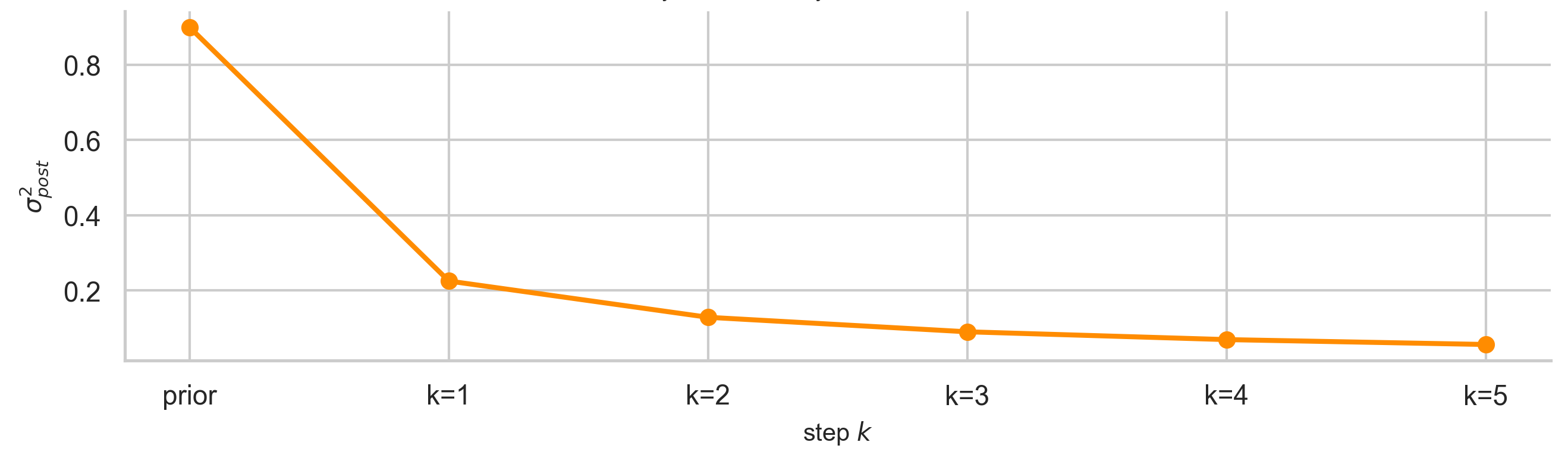
$$\frac{1}{\sigma_{post}^2} = \frac{1}{\sigma_0^2} + \frac{1}{\sigma_{obs}^2}$$

Precisions add. In the static case - one fixed truth, many observations - every observation makes you strictly more certain than before. Variance here is not merely uncertainty - it is a quantified expression of trust: how much should this source move my estimate? The update is a negotiation between two sources of information, weighted by how reliable each is believed to be. That weighting is what we will track across the rest of this post.

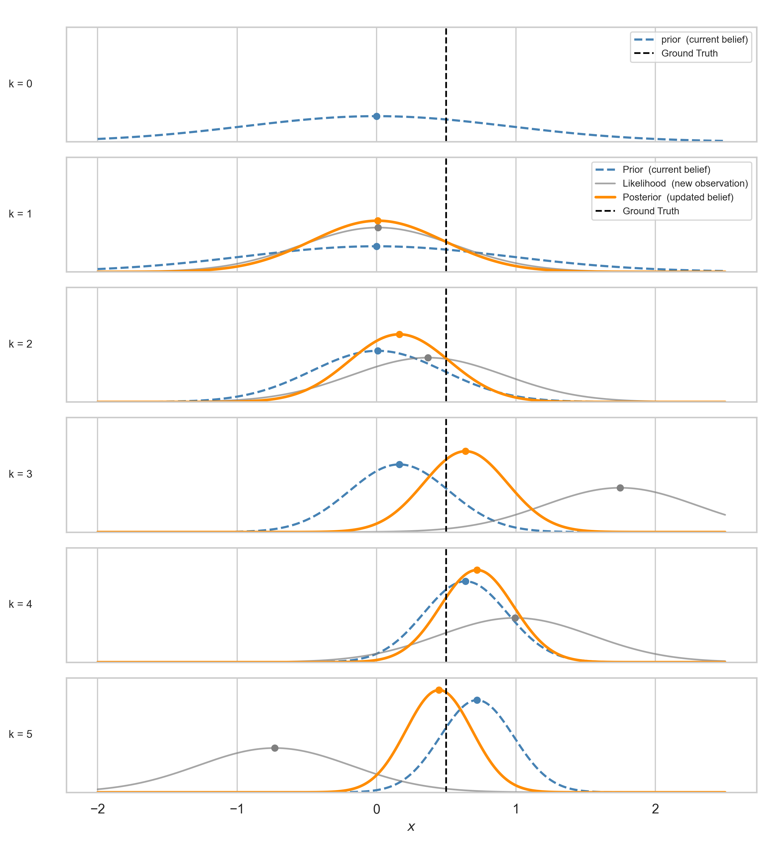
Applied sequentially, the posterior changes at each step $k$ like so:

For the “Actually…” Crowd: The Gaussian posterior minimises the KL divergence to the true posterior under quadratic structure: $KL(q(x) \| p(x \mid z))$. It is an information projection, not merely a weighted average.

This section describes what the optimal answer looks like. It says nothing about how to compute it in real time, on a world that evolves constantly. That is the next problem.

---

The Engineering Answer: The Kalman Filter

The Bayesian update above assumes the truth stays fixed. One value, many observations, converging belief. Rudolf Kalman’s 1960 paper ¹ asked what happens when it does not.

A drone drifting in wind. A satellite. A limb adapting to an unexpected load. The static assumption breaks immediately. (Yes, I am treating the world as linear-Gaussian for now. The nonlinear case is a different post.)

The state evolves according to:

$$x_{k} = A x_{k-1} + w_k, \qquad w_k \sim \mathcal{N}(0,\, Q)$$

$$z_{k} = C x_{k} + v_k, \qquad v_k \sim \mathcal{N}(0,\, R)$$

The first equation is the process model - how the state moves, corrupted by process noise $Q$. The second is the observation model - what the sensor sees, corrupted by measurement noise $R$.

The filter runs in two steps at every timestep:

$$\text{Predict:} \quad \hat{x}_k^- = A\hat{x}_{k-1}, \qquad P_k^- = A P_{k-1} A^T + Q$$$$\text{Update:} \quad K_k = \frac{P_k^-}{P_k^- + R}, \qquad \hat{x}_k = \hat{x}_k^- + K_k(z_k - C\hat{x}_k^-), \qquad P_k = (1 - K_k)P_k^-$$

The predict step is the filter acknowledging that time has passed - $Q$ inflates the covariance, uncertainty grows. The update step is the world pushing back - the observation prunes it. The filter lives in the tension between the two.

$K_k$ is the Kalman gain. When $P_k^-$ is large relative to $R$, the filter trusts the sensor. When $R$ dominates, it trusts the model. The same precision-weighting as before - same logic, new notation.

For the “Actually…” Crowd: The gain expression here is the 1D scalar case. In general, $K_k = P_k^- C^T (C P_k^- C^T + R)^{-1}$. The structure is the same — prior uncertainty weighted against observation noise — but the full form handles non-identity observation matrices. Also, at steady state, $K$ stops changing. The value of $P$ at which the predict step’s injection of $Q$ is exactly balanced by the update step’s reduction gives the discrete algebraic Riccati equation (DARE):

$$P_\infty = A P_\infty A^T + Q - A P_\infty C^T(C P_\infty C^T + R)^{-1} C P_\infty A^T$$

This is the dynamic counterpart of the static precision-addition formula from the Bayes section. The Riccati equation is Bayes’ theorem for a shifting world. Check out the appendix in the notebook if this is your thing! ^{2 3}

The Geometry of Belief, in Motion

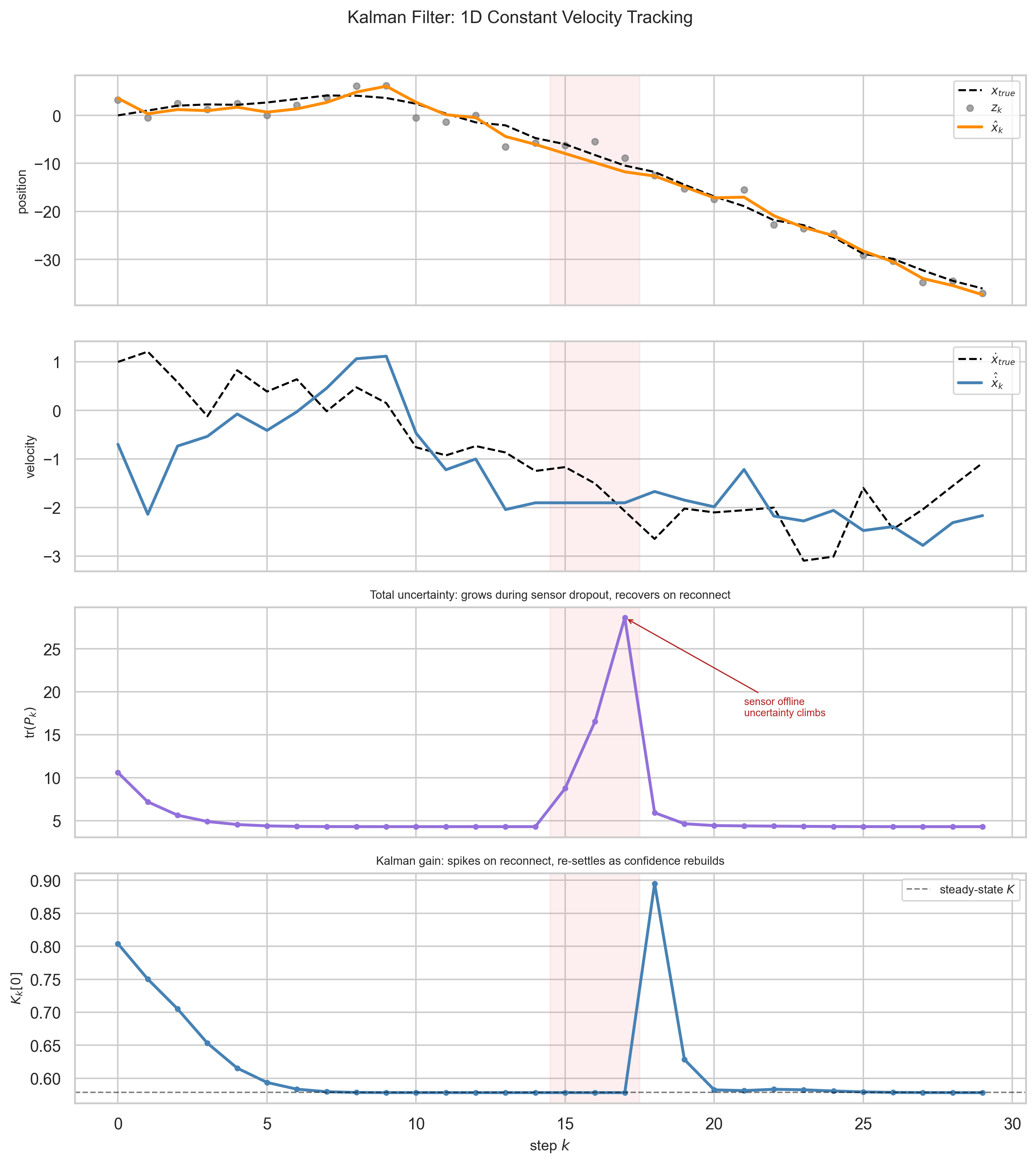
The filter starts with a bad prior - position off by five units, high initial uncertainty. It does not matter. Within a handful of steps, the estimate locks onto the true trajectory. High initial $P$ means high initial $K$ - the filter knows it does not know, and trusts the sensor heavily at first.

Velocity (panel 2) is never observed directly. It is inferred entirely from the pattern of position measurements and the process model. This is what “latent” means in practice - a quantity the system needs to track but never gets to see.

tr$(P_k)$ (panel 3) hits a floor - but not zero. The process noise $Q$ ensures the filter maintains a baseline of healthy uncertainty. When the sensor goes offline, uncertainty increases; when it reconnects, the filter snaps back. $K_k$ (panel 4) starts high and settles, spiking briefly on reconnection.

The Kalman filter is Bayes’ theorem with a prediction step shoved into the middle. As Särkkä (2013) notes, it is the simplest possible way to do Bayesian filtering in a world that refuses to sit still.

This is the engineering answer. It is provably optimal under linear-Gaussian assumptions. It runs recursively, online, at every timestep. It carries an explicit uncertainty estimate $P_k$ and adjusts how much it trusts new information in real time.

The question is whether anything like this is achievable under biological constraints. Not the matrices. Not the closed form. The architecture.

---

The Biological Answer: What Evolution Built Instead

This is where the argument gets harder - and more interesting.

The Impossible Engineering Brief

Imagine you are handed the following design brief: Build a system that predicts and corrects its own errors, in real time, from a single stream of experience, using only locally available information - with no replay, no global optimizer, and a hard millisecond deadline. There was no option for biology to refactor the physics, but rather, the system had to be correct enough to survive the next ten milliseconds, every ten milliseconds.

Before asking what the brain does, name the constraints it operates under.

No weight transport. Backpropagation requires passing error signals backward through the same weights used in the forward pass. No known biological projection works this way. The brain has to learn every synaptic update from local information only.

Millisecond timescales. Motor corrections begin before sensory feedback arrives.

No clean signal. The brain learns from a single continuous stream of experience, under stochastic spiking noise at every level. No replay, no held-out set, no second pass.

Any solution that works in this regime is, by engineering standards, remarkable. The question is not whether it matches the Kalman filter equation for equation. It is whether the architecture - predict, compute residual, weight the correction - survives in this substrate.

The architecture survives. And motor control is where the evidence is clearest.

Motor Control: The Existence Proof

Reach for a coffee cup. Your hand moves to the right location before your visual system has confirmed it got there. Your arm compensates for the weight of the cup before your muscles feel it. Corrections begin within 100ms of a perturbation - faster than a conscious response, and in many cases faster than sensory feedback can arrive.

How?

The brain maintains a forward model - an internal simulation of the body’s dynamics. Before a movement executes, the motor cortex sends a copy of the outgoing motor command - an efference copy - to the cerebellum. The cerebellum runs the command through its forward model and generates a prediction of the expected sensory consequence: the weight of the cup before your fingers close, the arc of your arm before proprioception confirms it. That prediction is the latent variable here - a belief about what should happen next, maintained and updated internally, never observed directly. When the actual sensory feedback arrives, the brain compares it to the prediction. The difference - the prediction error - drives learning and online correction.

This is predict-and-correct running in biological hardware, at millisecond resolution, with delay, without matrix inverses, without backpropagation, without a global loss function. The evidence is convergent across behavioral, anatomical, clinical, and computational lines.

Behavioral evidence. Motor adaptation follows a characteristic curve - rapid initial correction, gradual refinement, an after-effect when the perturbation is removed - that is quantitatively consistent with forward model updating. Interference between tasks, savings across sessions, and the specificity of generalization are all predicted by forward model accounts and not by simpler alternatives ⁴. The anatomical picture matches: the cerebellum receives efference copy via the pontine nuclei and returns predictive signals via the thalamus, structured exactly as a forward model requires ⁵. Patients with cerebellar lesions lose precisely the anticipatory component - their movements become reactive rather than predictive, which is the dissociation you would expect if a prediction mechanism were selectively removed ⁵.

Computational evidence. Wolpert’s MOSAIC framework ⁶ first formalized this as a bank of paired forward and inverse models, each weighted by how well it predicts the current context. Recent computational work such as Neural Adaptive Filter ⁷ generalizes the architecture further: a filter-controller framework that handles noisy observations and adapts online to unknown dynamics, connecting the motor control story directly to the estimation framing of this post. The biological constraints - no weight transport, millisecond timescales, no clean signal - leave very little room for how to solve the prediction-correction problem, and the structures that survive those constraints share a functional organization with the Kalman framework.

The implementation does not use matrix inverses or explicit gain schedules. The brain approximates precision-weighting through gain modulation, neuromodulatory signals, and the statistics of synaptic reliability. The mechanism is different. The function it computes is structurally the same.

Predictive Coding: The Generalization Attempt

Motor control is solid ground. Rao and Ballard (1999) ⁸ asked whether the same principle extends to perception itself - whether the visual cortex, like the cerebellum, is running a continuous prediction-error loop.

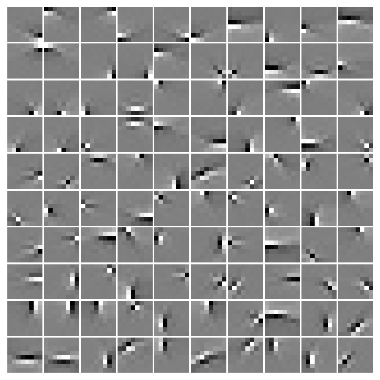
The idea: higher visual areas send top-down predictions to lower areas. Lower areas compute the residual and send the error back up. Neurons in lower areas are not feature detectors - they are error reporters. This reframing accounts for endstopping: V1 neurons that fire to a short bar but fall silent when it extends. A long bar is fully predicted; it generates no residual. A line termination is a surprise.

The stronger argument is a convergence result. Train a predictive coding model on natural images and it learns Gabor-like filters - the oriented edge detectors found in V1. Train a sparse autoencoder with no biological motivation and it learns the same filters ⁹. These are not identical models. But when the problem constrains the solution space tightly enough, different approaches under different pressures converge on the same structure. That is what “convergence” means here - not that all three found the same answer, but that the problem left very little room for alternatives.

What the model does not establish should be said plainly. The learning rule requires something functionally similar to weight transport - the same objection that applies to backpropagation applies here. The hierarchical architecture is schematic, not derived from known cortical connectivity. Predictive coding is a computational-level account in Marr’s sense: a description of what the system computes, not how it computes it.

The principle generalizes. The implementation remains open. These systems don’t share an equation. They share a problem - and the problem leaves very little room for how to solve it.

What Each Framework Knows - And What It Doesn’t

The three frameworks now sit next to each other - but not as equals wearing different coats. Each one is an answer to a different version of the same question, with different assumptions and different blind spots. They operate at different levels of description - normative, algorithmic, implementational - which is why collapsing them into a single table risks overstating the equivalence. What the table shows is not that these frameworks are the same object, but that they instantiate the same functional roles.

	Bayesian Inference	Kalman Filter	Biological Motor Control	Predictive Coding
The Prediction	Prior $\mu_{prior}$	State Estimate $C\hat{x}_k^-$	Efference copy forward model	Top-down $r_{td}$
The Residual	$\mu_{obs} - \mu_{prior}$	Innovation $z_k - C\hat{x}_k^-$	Sensory prediction error	Feedforward error signal
The Weight	Relative variance	Kalman Gain $K_k$	Gain modulation, neuromodulation	Precision $\Sigma^{-1}$ (speculative)
The Result	Posterior	Updated state estimate	Corrected motor command	Cortical representation
What it assumes	Static truth, Gaussian noise	Linear dynamics, known noise covariances	Local learning rules sufficient	Symmetric forward-backward connections
What it can’t do	Handle a moving world	Handle nonlinear dynamics exactly	Provide optimality guarantees	Confirm its own implementation

The $\sigma^2$ in a statistics textbook, the $P$ and $R$ matrices in Kalman’s 1960 paper, and the gain modulation signals in a cerebellar circuit are different implementations of the same function: deciding how much to trust the current observation relative to the current model.

That convergence is not a coincidence. It is what the constraint forces.

---

What AI Is Still Missing

Back to the language model and the benchmark. The common structure across all three frameworks is not prediction. It is that uncertainty is represented in the same space as the state, and directly controls how the state updates. That upstream-versus-downstream distinction is central.

Your LLM predicts well. What it does not do is maintain an explicit, updateable estimate of its own uncertainty about the current input - one that changes in real time as evidence accumulates and that distinguishes “I am uncertain because the input is ambiguous” from “I am uncertain because this input is unlike anything in my training distribution.”

The Kalman filter has $P_k$ - a covariance matrix that tracks how uncertain the estimate is right now, updated at every timestep. When the world is unpredictable (high $Q$), uncertainty grows. When the sensor is reliable (low $R$), the observation corrects it aggressively. The gain $K_k$ is a live signal that tells the system how much to trust what it just saw.

A transformer at inference time has no explicit, dynamically updated equivalent ¹⁰. The weights are frozen. There is no $P_k$. Attention weights and output entropy are proxies - they can signal that a distribution is peaked or flat, but they don’t feed back into how the next representation is formed. The model cannot distinguish a confident prediction from an overconfident one based on the structure of the current input alone - not in a way that changes the update, only in a way that changes the reported output.

The biological systems in Section 4 solve a structurally harder problem than pure next-token prediction. They predict the consequences of actions before the actions execute. They update their models online, from a single stream of experience, using only local signals. They modulate how much they trust each input based on context-dependent reliability signals. They do all of this under radical computational constraints that make gradient descent on a cluster look extravagant.

This is not an argument that transformers should be more brain-like. It is a more specific observation: the failure modes that currently matter most in deployed language models - hallucination, overconfidence on novel inputs, inability to express calibrated uncertainty - are precisely the failure modes you would expect from a system that has mastered prediction but treats uncertainty as an output rather than as a computational variable.

Conformal prediction, temperature scaling ¹¹, chain-of-thought hedging: these are all annotations on the output. None of them feeds back into how the next representation is formed. The architecture is untouched.

That is the structural gap. Not better calibration at the output. Not more data. A mechanism by which uncertainty over the current input is maintained, updated as context accumulates, and used to modulate how much that input shifts the model’s internal state. The three communities arrived at this independently because the problem leaves very little room for how to solve it. The question for AI is whether the same pressure - deploy systems that have to be right about what they don’t know, not just about what they do - will force the same convergence.

---

The Takeaway

The clearest test is behavioral: present the system with two inputs, one familiar and one genuinely out-of-distribution. If the internal representations would be identical regardless - if “how sure am I?” has no pathway to modulate the update - then uncertainty is downstream.

A Kalman filter fails this test usefully: the same observation can produce different updates depending on current $P_k$. A standard transformer always produces the identical hidden state for an identical token sequence.

Pressure is building toward architectures where uncertainty is a representational variable maintained and updated as part of the forward pass. State space models ¹², test-time adaptation ¹³, and online fine-tuning ¹⁴ explore pieces of this space, but many still update the wrong thing at the wrong granularity. The biological systems and the Kalman filter converged on this structure under very different constraints. Whether deployment pressures - hallucinations, overconfidence, distribution shift - will force AI architectures toward the same convergence remains open.

The argument of this post is that the pressure is real, the gap is structural, and the three communities already know what filling it looks like.

The next post examines what happens when you look at the transformer’s attention mechanism through this lens - what structural bets it makes, what it gives up, and why the architecture it replaced was a more serious opponent than the standard narrative admits.